
Code
import matplotlib.pyplot as plt
import numpy as np

cycler = plt.cycler("color", plt.cm.autumn(np.linspace(0, 1, 100)))
plt.rcParams["axes.prop_cycle"] = cyclerimport matplotlib.pyplot as plt
import numpy as np
cycler = plt.cycler("color", plt.cm.autumn(np.linspace(0, 1, 100)))
plt.rcParams["axes.prop_cycle"] = cyclerdef dpf_scholkman(
age: float or np.ndarray = 0.583, wavelength: float or np.ndarray = 760
) -> float or np.ndarray:
coefs = {
"alpha": 223.3,
"beta": 0.05624,
"gamma": 0.8493,
"delta": -5.723e-7,
"epsilon": 0.001245,
"zeta": -0.9025,
}
dpf = (
coefs["alpha"]
+ coefs["beta"] * (age ** coefs["gamma"])
+ coefs["delta"] * wavelength**3
+ coefs["epsilon"] * wavelength**2
+ coefs["zeta"] * wavelength
)
return dpfI have news! I’m starting my postdoc at the Institut de Recerca Hospital Sant Joan de Déu (Barcelona, Spain) in September, joining Chiara Santolin’s new research group. We will be carrying out experimental series as part of Chiara’s ERC project GaLa (Gates to Language). This project involves newborns, infants, rats, and some computational modelling to investigate early language acquisition and its evolutionary roots. I’ll be mostly involved with the neonates branch of the project, using fNIRS (functional near-infrared spectroscopy) to measure neonates’ brain response to different audio stimuli.
I’m new to fNIRS, so I was very lucky to spend two months at Prof. Emily Jones’ group at the Center of Brain and Cognitive Development (CBCD) at Birkbeck University (London, UK), and two weeks at Prof. Judit Gervain’s lab at Università di Padova. Folks at CBCD and in Padova were extremely generous with their time and knowledge, and after coming back from these research stays I feel like returning some of my time to the fNIRS community. I will dedicate some upcoming blog posts to some of my progress in learning fNIRS and the underlying theory and associated preprocessing piplines, with the aim of making the learning curve a bit less steep for future newcomers. In this blog post, I will provide a very simple Python function to calculate the Differential Pathlength Factor (DPF) for an individual, given their age and the specific wavelength used, following Scholkman’s method (Scholkmann & Wolf, 2013).
To estimate relative changes in concentration of HbO and HbR, most NIRS devices—particularly those that use a continuous wave (CW) system—shine a light into some tissue of interest at two wavelengths: one is more sensitive to changes in concentration of HbO, the other is more sensitive to changes in concentration of HbR. Light is shone from a source, travels through the tissue and is received by a detector. By estimating how much of the light gets attenuated, and by observing the spectral properties of the received light, NIRS provides an estimation of the presence of certain chromophores in the tissue (in our case, HbO and HbR). The modified Beer-Lambert Law (mBBL) (see Equation 1) describes how the light attenuation (\(A\)) changes for a particular wave length (\(\lambda\)):
\[ \Delta A = \varepsilon(\lambda) \cdot \Delta c \cdot d \cdot \text{DPF}(\lambda) \tag{1}\]
where \(\varepsilon\) is the extinction coefficient of a molecule at a certain wavelength, \(\lambda\) is the wavelength of the inyected light, \(c\) is the change in molecule concentration, \(d\) is the source-detector distance, and \(\text{DPF}\) is the differential pathlength factor. The DPF specifies the increment in photon path length due to scattering: sometimes, photons “bounce” against molecules also present in the medium, which increases the distance they travel through the biological tissues, ultimately influencing the intensity of the light that the detector receives at a particular wavelength. The DPF parameter takes a numeric value specified a priori by the researcher, based on prior knowledge about the properties of the tissue.
Conventional CW-based NIRS devices cannot determine exactly the true DPF, as this value is dependent on factors outside of the control or reach of the researcher. But some methods provide a reasonable approximation. One of them was presented by Scholkmann & Wolf (2013). The authors came up with an equation that takes into account the age of the participant, and the wavelength of the NIR light. These variables are then introduced in Equation 2:
\[ \text{DPF} (\lambda, A)= \alpha + \beta A ^{\gamma} + \delta \lambda ^{3} + \varepsilon \lambda ^{2} + \zeta \lambda \tag{2}\]
where \(\lambda\) is the wavelength, \(A\) is the age of the participant, and \(\alpha\), \(\beta\), \(\delta\), \(\varepsilon\), and \(\zeta\) are the certain coefficients that were empirically estimated by Scholkmann & Wolf (2013) using a robust nonlinear least squares method, based on previously published datasets. The result is a formula in which one can introduce the age of the participant and the wavelength of interest, and obtain the estimated DPF:
\[ \text{DPF} (\lambda, A)= 223.3 + 0.05624 A ^{0.8493} + −5.723 \times 10^{−7} \lambda ^{3} + 0.001245 \lambda ^{2} + −0.9025 \lambda \]
I made a simple Python function to implement the equation:
import matplotlib.pyplot as plt
import numpy as np
import matplotlib as mpl
def dpf_scholkman(
    age: float or np.ndarray = 0.583, wavelength: float or np.ndarray = 760
) -> float or np.ndarray:
    coefs = {
        "alpha": 223.3,
        "beta": 0.05624,
        "gamma": 0.8493,
        "delta": -5.723e-7,
        "epsilon": 0.001245,
        "zeta": -0.9025,
    }
    dpf = (
        coefs["alpha"]
        + coefs["beta"] * (age ** coefs["gamma"])
        + coefs["delta"] * wavelength**3
        + coefs["epsilon"] * wavelength**2
        + coefs["zeta"] * wavelength
    )
return dpfLet’s try it out:
age = 24  # years
wl = 760  # wavelength
dpf_scholkman(age, wl)6.122136155212161Let’s reproduce some of the figures in Scholkmann & Wolf (2013).
age = np.linspace(0, 50, 100)
wavelengths = np.linspace(690, 832, 100)
dpf = np.vstack([dpf_scholkman(age, w) for w in wavelengths])
fig, ax = plt.subplots(layout="constrained")
norm = mpl.colors.Normalize(vmin=np.min(wavelengths), vmax=np.max(wavelengths))
cycler = plt.cycler("color", plt.cm.autumn(np.linspace(0, 1, 100)))
x = np.vstack(np.array([age] * len(age))).transpose()
fig.colorbar(
    mpl.cm.ScalarMappable(norm=norm, cmap="autumn"),
    ax=ax,
    orientation="horizontal",
    location="top",
    label="Wavelength (nm)",
    aspect=30,
)
plt.rcParams["axes.prop_cycle"] = cycler
ax.plot(x, dpf.transpose())
ax.set_xlabel("Age (years)")
ax.set_ylabel("DPF")
ax.set_axisbelow(False)
ax.grid(color="gray", alpha=0.1)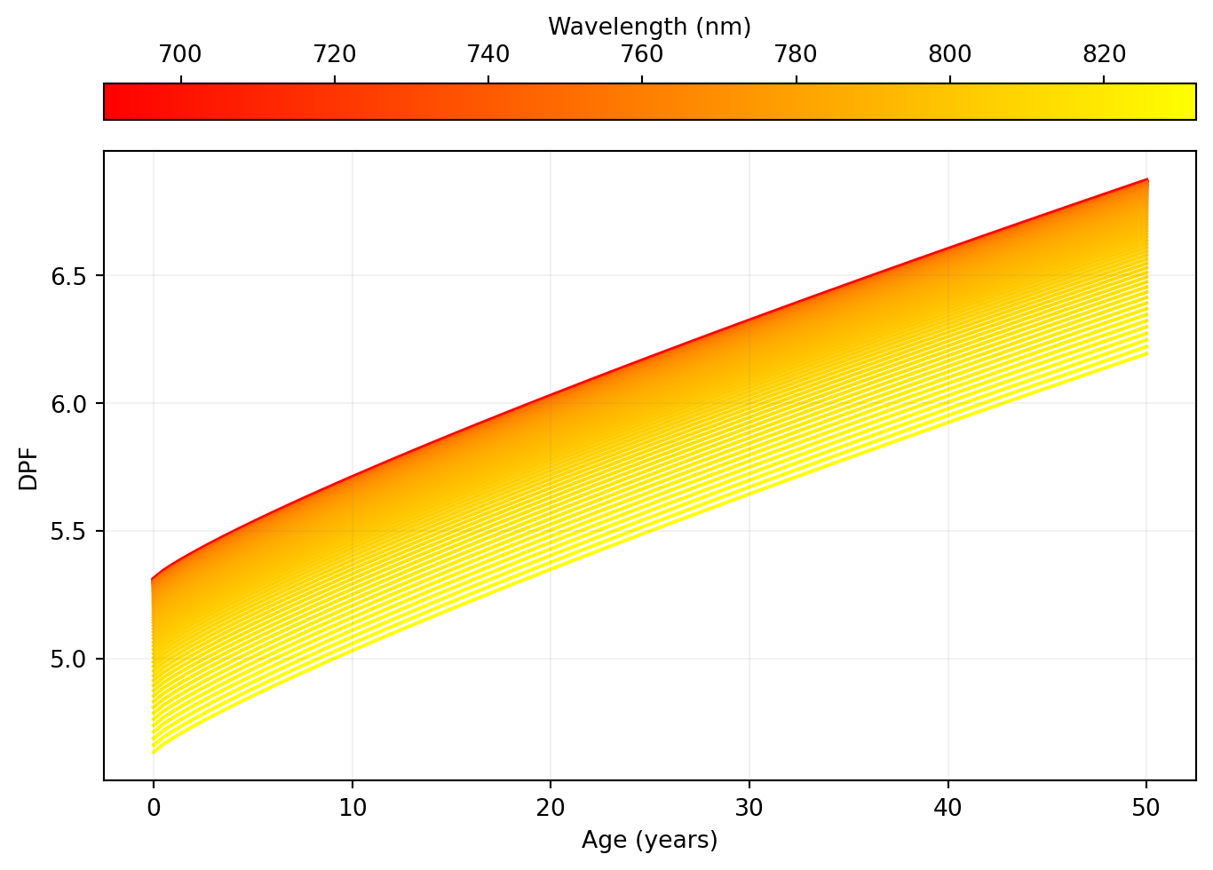
fig, ax = plt.subplots(layout="constrained")
norm = mpl.colors.Normalize(vmin=np.min(age), vmax=np.max(age))
cycler = plt.cycler("color", plt.cm.autumn(np.linspace(0, 1, 100)))
x = np.vstack(np.array([wavelengths] * len(wavelengths))).transpose()
fig.colorbar(
    mpl.cm.ScalarMappable(norm=norm, cmap="autumn"),
    ax=ax,
    orientation="horizontal",
    location="top",
    label="Age (years)",
    aspect=30,
)
plt.rcParams["axes.prop_cycle"] = cycler
ax.plot(x, dpf)
ax.set_xlabel("Wavelength (nm)")
ax.set_ylabel("DPF")
ax.set_axisbelow(False)
ax.grid(color="gray", alpha=0.1)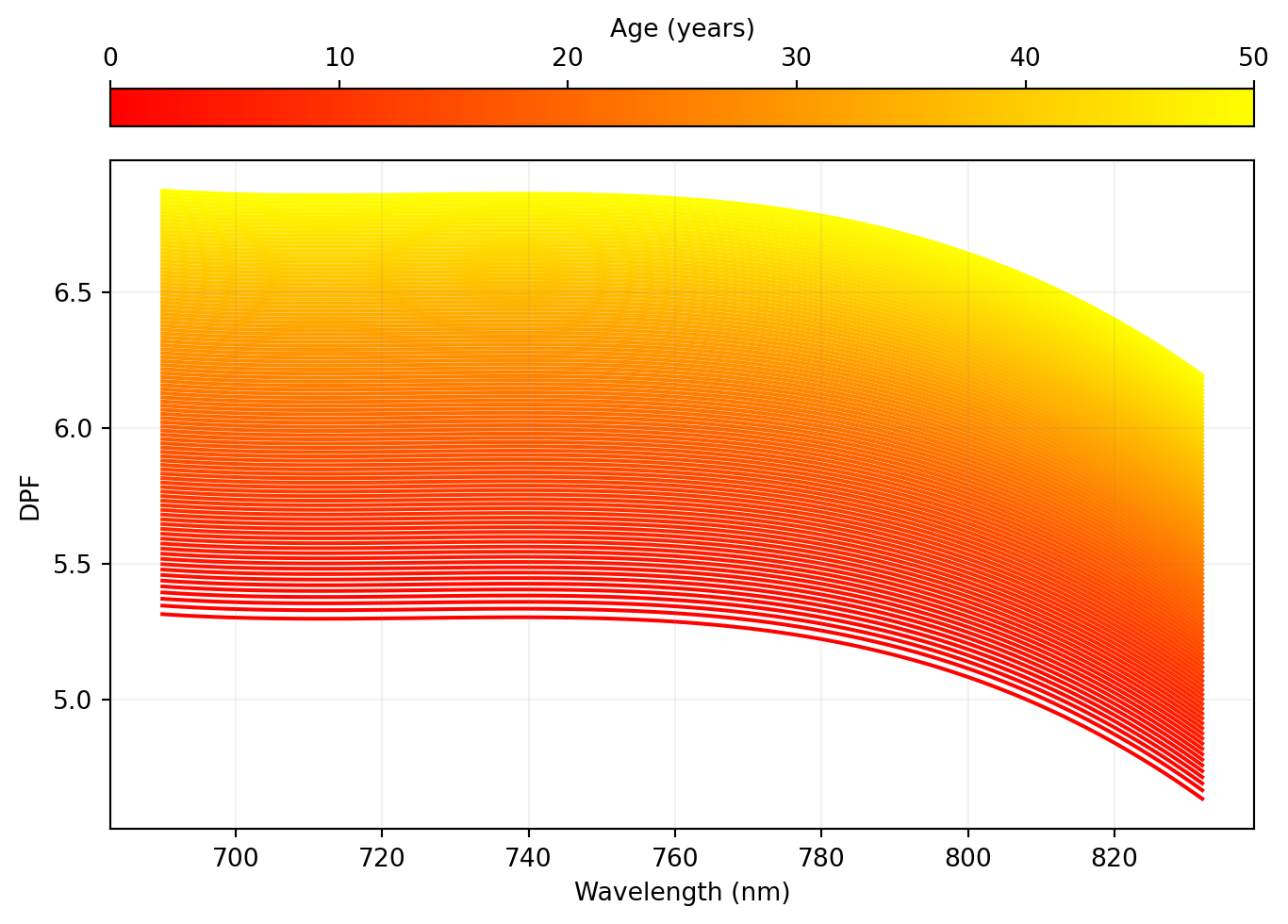
We can also visualise the behaviour of the DPF across ages and wavelengths as a 2D heatmap in Figure 3:
norm = mpl.colors.Normalize(vmin=np.min(dpf), vmax=np.max(dpf))

fig, ax = plt.subplots(layout="constrained")
ax.imshow(dpf.transpose(), cmap="autumn", aspect="auto")
ax.set_yticks(
    np.linspace(0, len(wavelengths), 10, dtype=int),
    labels=np.linspace(min(wavelengths), max(wavelengths), 10, dtype=int),
)
ax.set_xticks(
    np.linspace(0, len(age), 10, dtype=int),
    labels=np.linspace(min(age), max(age), 10, dtype=int),
)
fig.colorbar(
    mpl.cm.ScalarMappable(norm=norm, cmap="autumn"),
    ax=ax,
    orientation="horizontal",
    location="top",
    label="DPF",
    aspect=30,
)
ax.set_ylabel("Wavelength (nm)")
ax.set_xlabel("Age (years)")
ax.invert_yaxis()
ax.set_axisbelow(False)
ax.grid(color="gray", alpha=0.1)

plt.show()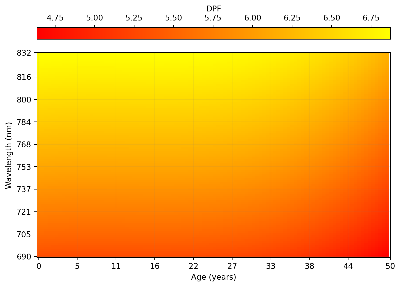
@online{garcia-castro2024,
  author = {Garcia-Castro, Gonzalo},
  title = {Implementing the {Differential} {Pathlength} {Factor} {(DPF)}
    in {Python:} The {Scholkmann} Method},
  date = {2024-11-24},
  url = {https://gongcastro.github.io/blog/dpf-scholkmann/dpf-scholkmann.html},
  langid = {en}
}